Introduction
On Twitter the other day, I tweeted “I always forget how much thinking goes into an RDA model.” Not a very profound tweet, but shortly after I received a message from someone new to statistical ordination techniques, and they asked me if I could share any resources I have regarding analysis and, specifically, interpretation of the results. For many of us starting out in research, learning new multivariate analyses can be confusing, daunting, and even trigger feelings of imposter syndrome. Fear not! With practice, lots of google searching, and using the resources available, you too can become an expert at multivariate ordinations. I was inspired to write a quick and dirty blog post meant for multivariate ordination newbies. In this post I discuss why multivariate ordinations are used, the different types of multivariate ordinations, and two examples of my own analyses and interpretation.
Why Multivariate Ordination?
In paleolimnology, I most often work with complex data consisting of many environmental variables (e.g. water temperature, conductivity, pH, etc.) as well as biological variables (e.g. species abundance data %). Multivariate ordination can be extremely useful for summarizing patterns in this high-dimensional data by reducing it down to a few low-dimensional axes or components. Multivariate ordination can also be used to test specific hypotheses related to your data. For example, I might ask which environmental gradients most influence diatom species abundance/distribution in a specific set of lakes. The type of ordination that you use is reliant on the data you have (qualitative vs. quantitative), the reason you are using it (patterns vs. hypothesis), and the length of your gradient.
Choosing Your Ordination Technique
This section draws from the Legendre & Birks Ch. 8 of Tracking Environmental Change Using Lake Sediments Volume 5 (contact me). It also draws from “Multivariate models” written by Abel Valdivia, which provides a wonderful overview of multivariate models along with a great example of multivariate analysis in R.
| Name | Acronym | Type | Algorithm | R Function | Use |
| Principle Components Analysis | PCA | Unconstrained | Eigenanalysis, SVD | stats::prcomp vegan::rda | Summarize patterns (preferred method) |
| Non-metric Multidimensional Scaling | NMDS | Unconstrained | Rank-order, distance based | vegan::metaMDS | Summarize patterns |
| Correspondence Analysis | CA | Unconstrained | RA, eigenanalysis, SVD | vegan::cca | Summarize patterns (preserve chi-squared distance |
| Detrended Correspondence Analysis | DCA | Unconstrained | RA with detrending and rescaling | vegan::decorana | Estimate length of gradient |
| Redundancy Analysis | RDA | Constrained | Eigenanalysis, SVD | vegan::rda | Hypothesis testing, summarize patterns |
| Canonical Correspondence Analysis | CCA | Constrained | Eigenanalysis, RA with regressions | vegan::cca | Hypothesis testing, summarize patterns |
In most cases, when summarizing patterns in multivariate data, PCA is the preferred method which preserves Euclidean distances and can be used on rather large datasets. Choosing your ordination technique is dependent on your data. There are a number of people that blog about this subject, and these posts are extremely helpful for understanding the work flow and thought process behind ordination analysis. I have compiled some links for each type of ordination to help you along with this process.
PCA – Principal Component Analysis (PCA) 101, using R by Peter Nistrup
PCA – Computing and visualizing PCA in R by Thiago G. Martins
PCA – vegan PCA: Principal Components Analysis with vegans rda function by Nathan Brouwer
PCA & NMDS – Introduction to Ordination by Koenraad van Meerbeek
NMDS – NMDS Tutorial in R by Jon Lefcheck
PCA, NMDS, CA, DCA, RDA, CCA – GUide to STatistical Analysis in Microbial Ecology (GUSTA ME) citation Buttigieg PL, Ramette A (2014) A Guide to Statistical Analysis in Microbial Ecology: a community-focused, living review of multivariate data analyses. FEMS Microbiol Ecol. 90: 543–550.
NMDS – Vegan Tutorial by Peter Clark
NMDS & CCA – Vegan: an introduction to ordination by Jari Oksansen
NMDS, PCA, CA, DCA, CCA – Multivariate Analysis of Ecological
Communities in R: vegan tutorial by Jari Oksansen
CA & CCA – Mosquito community diversity analysis with vegan by Randi H. Griffin
RDA – Session 5 Applied Multivariate Statistics RDA – demonstration in R by Ralf Schaefer
Principal Components Analysis (PCA) and Redundancy Analysis (RDA) Real World Examples
In this example, I use the vegan package in R to analyze diatom species abundance and physico-chemical environmental data from lakes in the Ecuadorian Andes. For this example, I will be using data from lakes in Cajas National Park.

Study Design
We sampled 8 lakes from Cajas National Park, southern Ecuador in July 2017. Diatoms were collected from the lake plankton using horizontal plankton tows along a transect from the center of each lake to the shore. Temperature, conductivity, and pH measurements were taken using a YSI microprobe. Water samples for analysis of major cations and anions were taken ~30 cm below the water surface, stored, and transported back to the US. Upon returning, diatoms were counted to >300 valves.
Description of the Data
First, load the libraries needed for the analysis.
#install packages DO THIS IN THE CONTROL PANEL!
install.packages(vegan)
install.packages(ggfortify)

#load libraries
library(vegan)
library(ggfortify)
library(faraway)
Next, import the data from GitHub
#import data from Github
 env <- read.csv("https://raw.githubusercontent.com/mluethje7/Cajas/main/CajasEnvironmental2017.csv", row.names=1)
 diatom <- read.csv("https://raw.githubusercontent.com/mluethje7/Cajas/main/CajasPlankton2017.csv", row.names=1)
There are two datasets here, one containing the environmental variables measured, and the other containing the diatom counts. It is important to explore and familiarize yourself with your data. In this case there are a few things to note. We have 8 different lakes or sites. There are a total of 107 diatom species variables (WOWZA) and 12 environmental variables that we will be investigating.
Data Transformations
Right now, the raw data needs to be prepared for statistical analysis through data transformations. First, the diatom counts need to be converted to relative abundance (%), and rare species (species <5% abundance) are removed. Rare species are removed because diatom community composition data often contains many 0 values since they have a unimodal response. Since we will be using ordination techniques, the diatom abundance data will be transformed once more using the Hellinger transformation to accommodate linear assumptions as recommended by Legendre & Gallagher 2001.
#tranform raw diatom counts to relative abundance
diatom <- diatom/rowSums(diatom)*100

#removal of rare species
abund <- apply(diatom, 2, max)
n.occur <- apply(diatom>0, 2, sum)
D <- diatom[, n.occur >2 & abund>5]

#Hellinger transformation
D <- decostand(D, method = "hellinger")
Now, we need to consider the environmental variables. First, evaluate the environmental variables by examining their distribution. Are they normally distributed? The variables we are working with are not the same units and are not all normally distributed, and thus need to be standardized. These variables are going to be log transformed to fit assumptions of linearity and homogenization.
#example of exploring environmental variable distribution
par(mfrow=c(1,2))
hist(env$Zmax, breaks = 5, col = "pink", xlab = "Max Depth (m)", main = "Histogram Max Depth")
hist(env$Water.T, breaks = 5, col = "pink3", xlab = "Temperature (C)", main = "Histogram Temperature")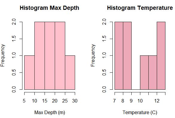
#log transformation of all variables except pH
E <- transform(env, Water.T=log10(Water.T+0.25), Cond=log10(Cond+0.25),
                 Secchi=log10(Secchi+0.25), Ca=log10(Ca+0.25), Mg=log10(Mg+0.25), K=log10(K+0.25),
                 SO4=log10(SO4+0.25), TN=log10(TN+0.25), Na=log10(Na+0.25), Cl=log10(Cl+0.25))
Now the data are ready for ordination! YIPPEEE SKIPPEEE!
Principal Components Analyses (PCA)
We will be exploring both data sets individually first using PCA. This is meant to summarize the patterns in the data. This can help us determine variables that are correlated with one another and sites that are most similar to one another.
#PCA using diatom species
pca1 <- prcomp(D, scale = TRUE) ##perform PCA
summary(pca1) ##calls a summary of the results
autoplot(pca1, label = TRUE, shape = FALSE, loadings = TRUE, loadings.label = TRUE, loadings.color = "blue", loadings.label.color = "blue", scale = 0) ##plots the pca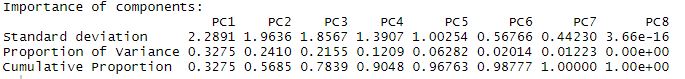
The summary shows us the breakdown of the components. The proportion of variance shows us how much variation is explained by that axis. So for PC1, 32.75% of the variance is explained, while for PC2, 24.1% of the variance is explained. This means the first two axes have captured ~56% of the total unconstrained variance.
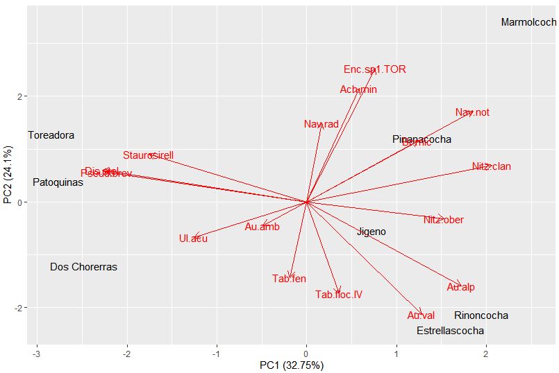
We can quickly plot up these results with the autoplot function. Sites are given scores for each PC axis. For example, Dos Chorerras has a PC1 score of -2.4 and a PC2 score of -1.2. Each species also receives a score relating to each PC axis. On this plot, the arrows point to the direction on the plot in which that species abundance would be increasing. The specific species scores can be found below.
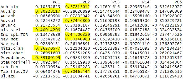
Note, for PC1 the most negative values correspond to Discostella stelligera and Pseudostaurosira, with the more positive values belong to Nitzschia clandestina and Aulacoseira alpigena. So lakes on the plot, like Dos Chorerras, Toreadora, and Patoquinas which have more positive site scores contain a higher abundance of the D. stelligera and Pseudostaurosira; while lakes with more negative scores have higher abundances of A. alpigena and N. clandestina. What can you find for PC2?
We can do the same process to explore the environmental variables. Let’s see what we find.
#PCA using environmental variables
pca2 <- prcomp(E, scale = TRUE) ##perform PCA
summary(pca2) ##calls a summary of the results
autoplot(pca2, label = TRUE, shape = FALSE, loadings = TRUE, loadings.label = TRUE, loadings.color = "blue", loadings.label.color = "blue", scale = 0) ##plots the pca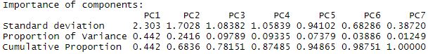
Again the summary shows us the breakdown of the components. Here, PC1 explains 44.2% of the total variance, and PC2 explains 24.16% of the total variance.
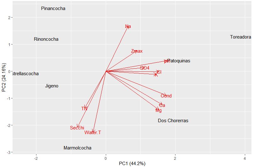
We can again analyze the plot to look at patterns in the data. PC1 is heavily influenced by pH, conductivity, and associated ions (Ca, K, Mg). While PC2 is influenced by water temperature, Secchi transparency, sodium content, and depth. So now how do these environmental variables relate to our species data? We have a perfect opportunity to try constrained ordination!
Redundancy Analysis (RDA)
RDA determines the variance in a set of response variables (species) that can be explained by a set of explanatory variables (environmental). Prior to performing the RDA, we need to further evaluate the data! Yes, I know, more work. In order for RDA to function correctly, you must have less explanatory variables than you have sites or your dataset is over constrained. Therefore, we must eliminate explanatory variables that are highly correlated.
#Evaluate correlation in environmental data
#Create correlation panel courtesy of youtube tutorial
panel.cor <- function(x, y, digits=2, prefix="", cex.cor)
 {
   usr <- par("usr"); on.exit(par(usr))
   par(usr = c(0,1,0,1))
   r <- abs(cor(x, y, use="complete.obs"))
   txt <- format(c(r, 0.123456789), digits=digits)[1]
   txt <- paste(prefix, txt, sep="")
   if(missing(cex.cor)) cex <- 0.8/strwidth(txt)
 test <- cor.test(x,y)
   # borrowed from printCoefmat
   Signif <- symnum(test$p.value, corr = FALSE, na = FALSE,
                    cutpoints = c(0, 0.5, 0.1, 1),
                    symbols = c("*", ".", " "))
 text(0.5, 0.5, txt, cex = cex * r)
   text(.8, .8, Signif, cex=cex, col=2)
 }

#Make full panel
pairs(E, lower.panel = panel.smooth, upper.panel = panel.cor)
This creates a rather large panel of your environmental variables, their correlations, and the significance of those correlations.
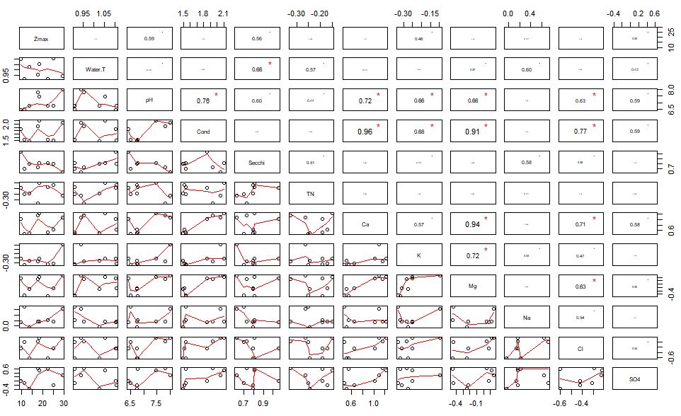
We can see that conductivity is related to a number of other variables including Ca, K, Mg, and Cl. Since conductivity is related to each of these individual cations – we can remove the cations from the analysis. I am crap at sub-setting still, but you can remove these variables from you dataset by individual column using the following function.
#remove columns
E <- E[,-7] #removes Ca, K, and Mg
E <- E[,-8] #removes Cl
You will have to make some choices in your data while doing this process. You may even try the RDA model multiple different times to find the most significant model and the overall best outcome from your data. As you do this, check the variance inflation factor (VIF). The VIF is a measure of the amount of multicollinearity in a set of multiple regression variables. Variables with a VIF >10 should be avoided. For this model, I have chosen to use water temperature, pH, conductivity, and TN. I chose these because I am most interested in these specific variables, and they influence other ones that they are correlated with (e.g. conductivity and cations/anions)
#check variance inflation factors (VIF)
sort(vif(E))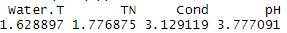
Now we must make sure that the length of our gradient is adequate for RDA using detrended correspondence analysis (DCA). If the gradient length is >4 it is more suitable for CCA.
#DCA species gradient
decorana(D, iweigh=1)
The axis length is 1.9, and is therefore less than 4 so we can continue on with our RDA model.
#RDA full model
rda <- rda(D ~ ., data = E) ## all explanatory variables
summary(s_rda)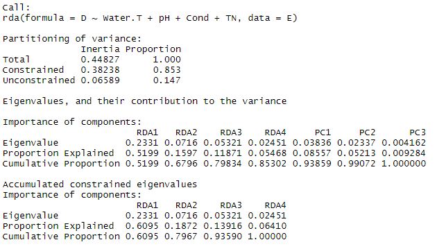
The summary will pop up the results above. The total variance is broken down into constrained and unconstrained components. In this global model, our explanatory variables explain 85.3% of the total variance, and there is 14.7% unconstrained. This means we have captured a pretty high percentage of the variance here with our explanatory data set. There are four constrained RDA axes, and three unconstrained PC axes.
We can test the significance of this model.
#test significance of global model
set.seed(111)
anova.cca(rda, step = 1000) 
The significance test suggests that our full model is statistically significant. You can also look at which axes contribute most to this significance.
#axis significance
anova.cca(rda, by="axis", step = 1000)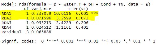
Now we can take a look at the RDA triplot
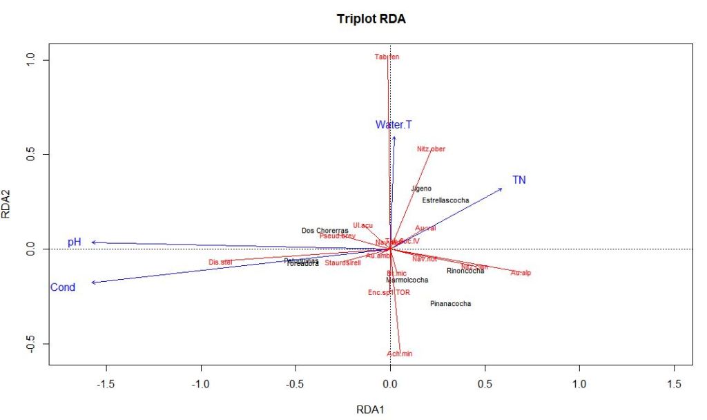
You can evaluate which environmental variables are most influential for each axis in the same way you did for PCA.
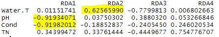
Here, pH and conductivity are pulling the first axis, and thus must be pretty influential on our diatom species composition. Water temperature and to a lesser extent TN are associated with RDA2. Lakes with lower scores on the RDA1 axis have higher pH and higher conductivity. Discostella stelligera abundance appears to be associated with pH and conductivity in this subset of lakes.
Assuming your model does not test significantly on the first try, you can use forward model selection using the ordistep() function. I highly suggest watching the RDA YouTube video tutorial for further help on this subject.
Final Comments
This is my first ever blog post related to statistics. I am aware I may have missed some steps. If you have any questions feel free to contact me and I would be happy to discuss. I also welcome any kind constructive criticism or suggestions. Thanks for reading!
